central_group — central_group • fonctionr

Function to compare means or medians among different groups based on complex survey data. It produces a list containing a table, including the confidence intervals of the indicators, a ready-to-be published ggplot graphic and a statistical test.

In case of mean comparison, the statistical test is a Wald test (using survey::regTermTest()). In case of median comparison the statistical test is a Kruskal Wallis test (using survey::svyranktest()). The confidence intervals and the statistical test are taking into account the complex survey design. In case of facets, the statistical test is computed on the total means or medians between facets (and not within facets). In case of second group (group.fill), no statistical test is computed.

Exporting the results to an Excell file is possible.

Usage

central_group(
  data,
  group,
  quanti_exp,
  type,
  group.fill = NULL,
  facet = NULL,
  filter_exp = NULL,
  ...,
  na.rm.group = TRUE,
  na.rm.facet = TRUE,
  total = TRUE,
  reorder = FALSE,
  show_ci = TRUE,
  show_n = FALSE,
  show_value = TRUE,
  show_labs = TRUE,
  total_name = NULL,
  digits = 0,
  unit = "",
  dec = NULL,
  col = NULL,
  pal = "OBSS_Spring",
  direction = 1,
  desaturate = 0,
  lighten = 0,
  darken = 0,
  dodge = 0.9,
  font = "Roboto",
  wrap_width_y = 25,
  wrap_width_leg = 25,
  legend_ncol = 4,
  title = NULL,
  subtitle = NULL,
  xlab = NULL,
  ylab = NULL,
  legend_lab = NULL,
  caption = NULL,
  lang = "fr",
  theme = "fonctionr",
  coef_font = 1,
  export_path = NULL
)

median_group(..., type = "median")

mean_group(..., type = "mean")

Arguments

data: A dataframe or an object from the survey package or an object from the srvyr package.
group: A variable defining groups to be compared.
quanti_exp: An expression defining the quantitative variable from which the mean/median is computed. Notice that if any observations with NA in at least one of the variable in quanti_exp are excluded for the computation of the indicators.
type: "mean" to compute mean by group ; "median" to compute median by group.
group.fill: A variable defining a second variable of groups to be compared.
facet: A variable defining the faceting group.
filter_exp: An expression filtering the data, preserving the design. Notice that filter_exp works as srvyr::filter(): it excludes observations for which filter_exp results into NA. It is often the case when NA is present on one of the filter variables.
...: All options possible in srvyr::as_survey_design().
na.rm.group: TRUE if you want to remove observations with NA on the group and the group.fill variables. FALSE if you want to create a group with the NA values for the group variable and a group.fill with the NA values for the group.fill variable. Default is TRUE.
na.rm.facet: TRUE if you want to remove observations with NA on the facet variable. FALSE if you want to create a facet with the NA values for the facet variable. Default is TRUE.
total: TRUE if you want to compute a total, FALSE if you don't. The default is TRUE.
reorder: TRUE if you want to reorder the groups according to the mean/median. NA value, if na.rm.group = FALSE, is not included in the reorder. In case of facets, the groups are reordered based on each median group. Default is FALSE.
show_ci: TRUE if you want to show the error bars on the graphic. FALSE if you don't want to show the error bars. Default is TRUE.
show_n: TRUE if you want to show on the graphic the number of observations in the sample in each group. FALSE if you don't want to show this number. Default is FALSE.
show_value: TRUE if you want to show the mean/median in each group on the graphic. FALSE if you don't want to show the mean/median. Default is TRUE.
show_labs: TRUE if you want to show axes and legend (in case of a group.fill) labels. FALSE if you don't want to show any labels on axes and legend. Default is TRUE.
total_name: Name of the total displayed on the graphic. Default is "Total" in French and in English and "Totaal" in Dutch.
digits: Number of decimal places displayed on the values labels on the graphic. Default is 0.
unit: Unit displayed on the graphic. Default is none ("").
dec: Decimal mark displayed on the graphic. Default depends on lang: "," for fr and nl ; "." for en.
col: Color of the bars if there is no group.fill. col must be a R color or an hexadecimal color code. Default color used depends on type : "deeppink3" for mean and "mediumorchid3" for median. The colors of total and NA group (in case of na.rm.group = FALSE) are always "grey40" and "grey". If there is a group.fill, col has no effect and pal argument should be used instead.
pal: Colors of the bars if there is a group.fill. pal must be vector of R colors or hexadecimal colors or a palette from packages MetBrewer or PrettyCols or a palette from fonctionr. The color of missing values for group.fill (in case of na.rm.group = FALSE) and for the total are always "grey" and "grey40". If there is no group.fill, pal has no effect and col argument should be used instead.
direction: Direction of the palette color. Default is 1. The opposite direction is -1. If there is no group.fill, this argument has no effect.
desaturate: Numeric specifying the amount of desaturation where 1 corresponds to complete desaturation (no colors, grey layers only), 0 to no desaturation, and values in between to partial desaturation. Default is 0. It affects only the palette (pal, if there is a second group) and not the monocolor (col, if there is no second group). See colorspace::desaturate function from colorspace package for details. If desaturate and lighten/darken arguments are used, lighten/darken is applied in a second time (i.e. on the color transformed by desaturate).
lighten: Numeric specifying the amount of lightening. Negative numbers cause darkening. Value shoud be ranged between -1 (black) and 1 (white). Default is 0. It doesn't affect the color of NA (in case of na.rm.group = FALSE). It affects only the palette (pal, if there is a second group) and not the monocolor (col, if there is no second group). See colorspace::desaturate for details. If both argument ligthen and darken are used (not advised), darken is applied in a second time (i.e. on the color transformed by lighten).
darken: Numeric specifying the amount of lightening. Negative numbers cause lightening. Value shoud be ranged between -1 (white) and 1 (black). Default is 0. It doesn't affect the color of NA (in case of na.rm.group = FALSE). It affects only the palette (pal, if there is a second group) and not the monocolor (col, if there is no second group). See colorspace::desaturate for details. If both argument ligthen and darken are used (not advised), darken is applied in a second time (i.e. on the color transformed by lighten).
dodge: Width of the bars. Default is 0.9 to let a small space between bars. A value of 1 leads to no space betweens bars. Values higher than 1 are not advised because they cause an overlaping of the bars. dodge doesn't affect the spaces between second groups (group.fill). There is always no space between second groups.
font: Font used in the graphic. See load_and_active_fonts() for available fonts. Default is "Roboto".
wrap_width_y: Number of characters before going to the line for the labels of the groups. Default is 25.
wrap_width_leg: Number of characters before going to the line for the labels of the group.fill. Default is 25.
legend_ncol: Number of columns in the legend. Default is 4.
title: Title of the graphic.
subtitle: Subtitle of the graphic.
xlab: X label on the graphic. As ggplot2::coord_flip() is used in the graphic, xlab refers to the x label on the graphic, after the ggplot2::coord_flip(), and not to the x variable in the data. Default (xlab = NULL) displays, for type = "mean", "Moyenne :" (if lang = "fr"), "Mean:" (if lang = "en") or "Gemiddelde:" (if lang = "nl"), or, for type = "median", "Médiane :" (if lang = "fr"), "Median:" (if lang = "en") or "Mediaan:" (if lang = "nl"), followed by the quanti_exp argument. To show no X label, use xlab = "".
ylab: Y label on the graphic. As ggplot2::coord_flip() is used in the graphic, ylab refers to the y label on the graphic, after the ggplot2::coord_flip(), and not to the y variable in the data. Default (ylab = NULL) displays the name of the group variable. To show no Y label, use ylab = "".
legend_lab: Legend (fill) label on the graphic. If legend_lab = NULL, legend label on the graphic will be group.fill. To show no legend label, use legend_lab = "".
caption: Caption of the graphic. This caption goes under de default caption showing the result of the statistical test. There is no way of not showing the result of the chi-square test as a caption.
lang: Language of the indications on the graphic. Possibilities are "fr" (french), "nl" (dutch) and "en" (english). Default is "fr".
theme: Theme of the graphic. Default is "fonctionr". "IWEPS" adds y axis lines and ticks. NULL uses the default grey ggplot2 theme.
coef_font: A multiplier factor for font size of all fonts on the graphic. Default is 1. Usefull when exporting the graphic for a publication (e.g. in a Quarto document).
export_path: Path to export the results in an xlsx file. The file includes three (without group.fill) or two sheets (with a group.fill): the table, the graphic and the statistical test result.

Value

A list that contains a table, a ggplot graphic and, in most cases, a statistical test.

Examples

# Loading of data
data(eusilc, package = "laeken")

# Creation of age categories
eusilc$age_cat <- cut(eusilc$age,
breaks = 6,
include.lowest = TRUE)

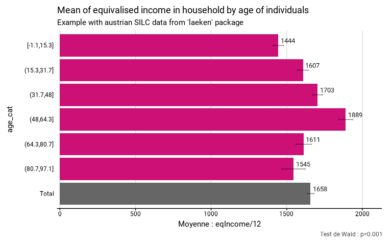
# Calculation of income means by age category with fonctionr, taking sample design into account
eusilc_mean <- mean_group(
  eusilc,
  group = age_cat,
  quanti_exp = eqIncome / 12,
  strata = db040,
  ids = db030,
  weight = rb050,
  title = "Mean of equivalised income in household by age of individuals",
  subtitle = "Example with austrian SILC data from 'laeken' package"
)
#> Input: data.frame
#> Sampling design -> ids:  db030, strata:  db040, weights:  rb050
#> Variable(s) detected in quanti_exp: eqIncome
#> Numbers of observation(s) removed by each filter (one after the other): 
#> 0 observation(s) removed due to missing group
#> 0 observation(s) removed due to missing value(s) for the variable(s) in quanti_exp

# Results in graph form
eusilc_mean$graph
#> Warning: Removed 6 rows containing missing values or values outside the scale range
#> (`geom_text()`).
#> Warning: Removed 1 row containing missing values or values outside the scale range
#> (`geom_text()`).


# Results in table format
eusilc_mean$tab
#> # A tibble: 7 × 8
#>   age_cat      mean mean_low mean_upp n_sample n_weighted n_weighted_low
#>   <fct>       <dbl>    <dbl>    <dbl>    <int>      <dbl>          <dbl>
#> 1 [-1.1,15.3] 1444.    1409.    1479.     2720   1424958.       1358818.
#> 2 (15.3,31.7] 1607.    1571.    1643.     2944   1612502.       1549489.
#> 3 (31.7,48]   1703.    1669.    1737.     4025   2230581.       2163723.
#> 4 (48,64.3]   1889.    1843.    1935.     2817   1578046.       1517273.
#> 5 (64.3,80.7] 1611.    1561.    1662.     1847   1053098.       1001605.
#> 6 (80.7,97.1] 1545.    1467.    1622.      474    283037.        256754.
#> 7 Total       1658.    1635.    1681.    14827   8182222        8079226.
#> # ℹ 1 more variable: n_weighted_upp <dbl>