Couleurs pour l'Observatoire de la Santé et du Social • fonctionr

Nous avons créé des palettes spécifiques pour les chercheurs de l’Observatoire de la Santé et du Social. Celles-ci suivent le code couleur de Vivalis, et ont été pensées pour différentes utilisations.

Utilisation

Pour utiliser ces palettes dans les différentes fonctions de fonctionr, il suffit d’indiquer celle de votre préférence (les noms des palettes de couleur sont listés plus loin sur cette page) dans l’argument pal :

test_palette_OBSS <- distrib_group_d(
  eusilc,
  group = db040,
  quali_var = pl030_rec,
  weights = rb050,
  font = "Gotham Narrow",
  pal = "OBSS",
  title = "Distribution of socio-economic status according to region",
  ylab = "",
  legend_lab = "Status",
  caption = "Bron : EU-SILC",
)
test_palette_OBSS$graph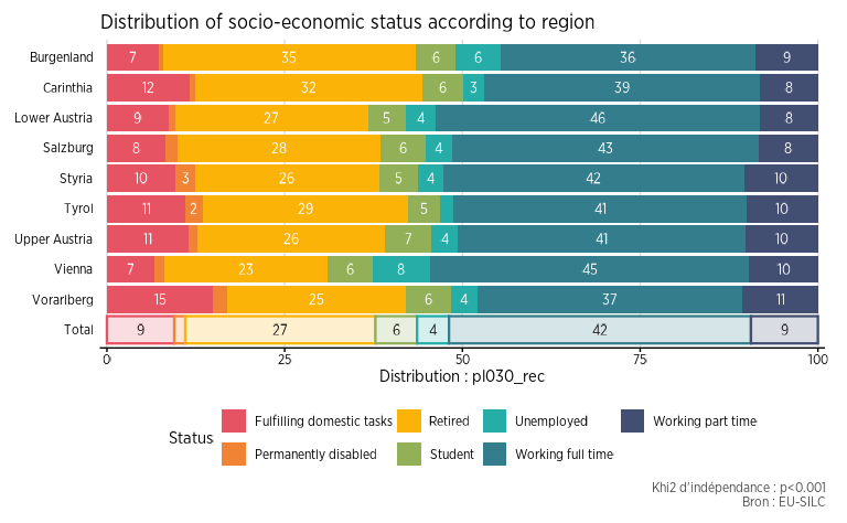

Les codes hexadécimaux des différentes palettes peuvent aussi être appelés avec la fonction official_pal(), pour les utiliser à l’extérieur de fonctionr. L’argument n permet d’indiquer combien de couleurs sont nécessaires, et la fonction s’occupe de créer automatiquement un dégradé comprenant ce nombre de couleurs. L’argument show_pal = T permet quant à lui d’afficher graphiquement les palettes.

official_pal(inst = "OBSS", n = 8)
#> [1] "#E65362" "#EF7C3B" "#F8A514" "#BEB135" "#63AE7A" "#2A9FA0" "#367689"
#> [8] "#434E73"
official_pal(inst = "OBSS", n = 8, show_pal = T)

Il est également possible de connaître toutes les palettes disponibles en exécutant la fonction official_pal() avec comme argument list_pal_names = T :

official_pal(list_pal_names = T)
#>  [1] "Vivalis"         "OBSS"            "OBSS_alt1"       "OBSS_alt2"      
#>  [5] "OBSS_alt3"       "OBSS_Relax"      "OBSS_Autumn"     "OBSS_Sweet"     
#>  [9] "OBSS_Spring"     "OBSS_Candy"      "OBSS_Greens"     "OBSS_Sea"       
#> [13] "OBSS_Sunset"     "OBSS_Purples"    "OBSS_Blues"      "OBSS_Brown"     
#> [17] "OBSS_div_mid1"   "OBSS_div_mid2"   "OBSS_div_mid3"   "OBSS_div_mid4"  
#> [21] "OBSS_div_bi1"    "OBSS_div_bi2"    "OBSS_div_bi3"    "OBSS_div_bi4"   
#> [25] "OBSS_highlight1" "OBSS_highlight2" "OBSS_highlight3" "OBSS_old"       
#> [29] "IBSA"            "ULB"

Les palettes

Palettes qualitatives

official_pal("OBSS", 8, show_pal = T)

official_pal("OBSS_alt1", 8, show_pal = T)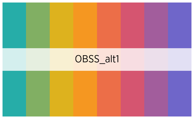

official_pal("OBSS_alt2", 7, show_pal = T)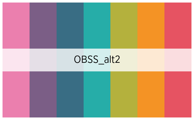

official_pal("OBSS_alt3", 8, show_pal = T)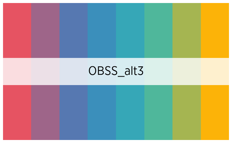

official_pal("OBSS_Autumn", 8, show_pal = T)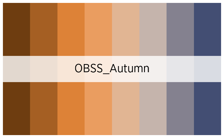

official_pal("OBSS_Relax", 7, show_pal = T)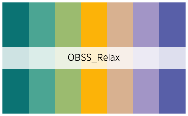

official_pal("OBSS_Spring", 7, show_pal = T)

official_pal("OBSS_Sweet", 7, show_pal = T)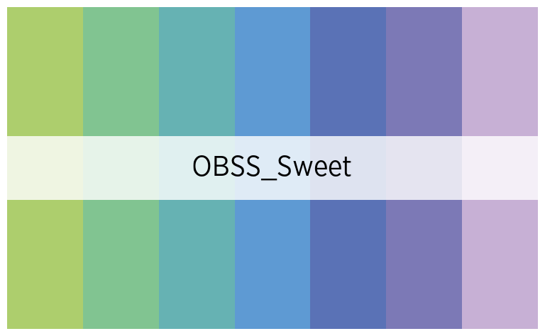

Palettes continues

official_pal("OBSS_Greens", 8, show_pal = T)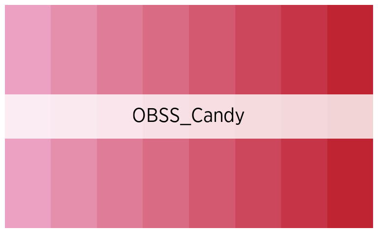

official_pal("OBSS_Sunset", 8, show_pal = T)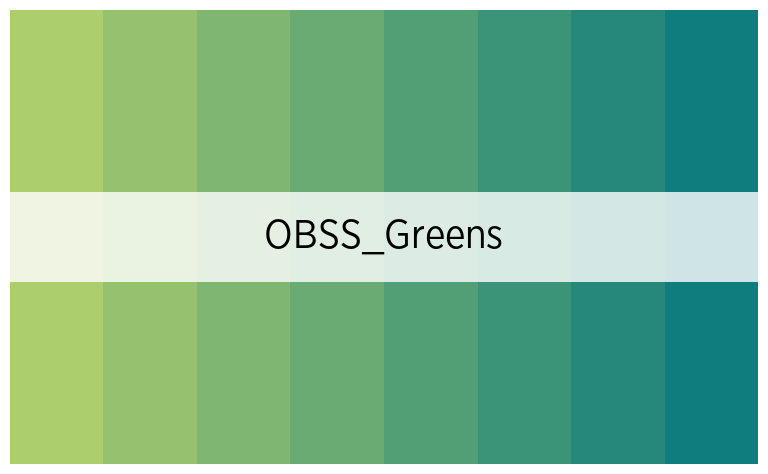

official_pal("OBSS_Sea", 8, show_pal = T)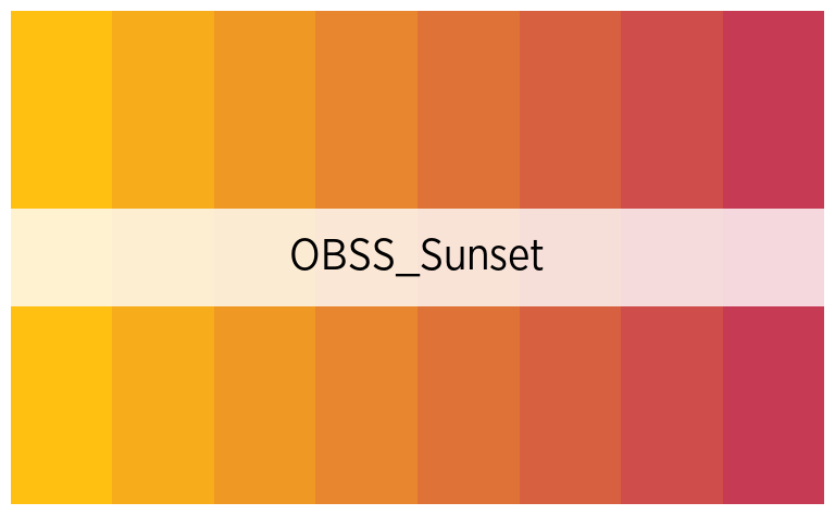

official_pal("OBSS_Candy", 8, show_pal = T)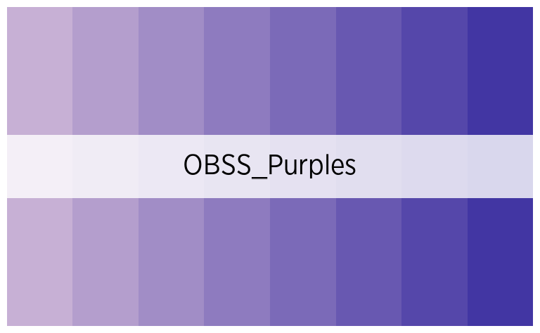

official_pal("OBSS_Purples", 8, show_pal = T)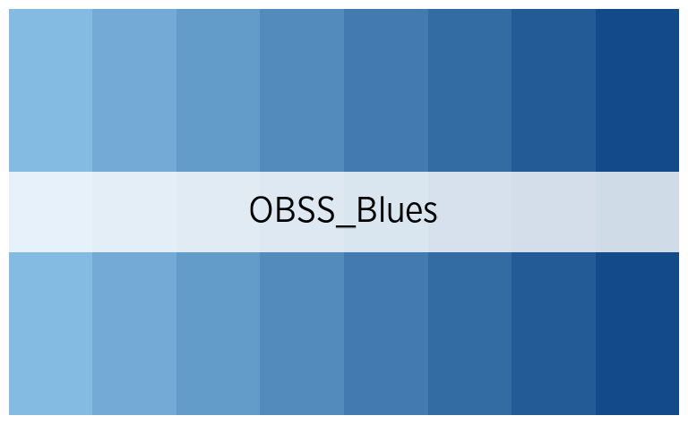

official_pal("OBSS_Blues", 8, show_pal = T)

official_pal("OBSS_Brown", 8, show_pal = T)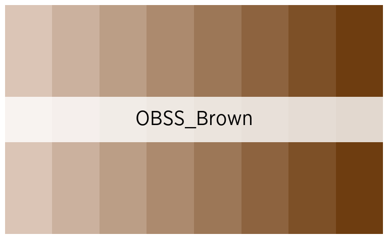

Palettes divergentes

Avec un point central

Attention, ces palettes n’affichent le point central que si le nombre de couleur est impair !

official_pal("OBSS_div_mid1", 7, show_pal = T)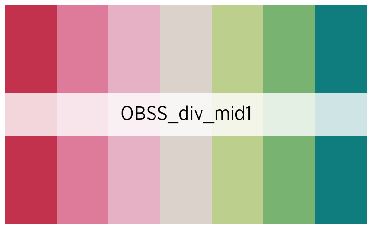

official_pal("OBSS_div_mid2", 7, show_pal = T)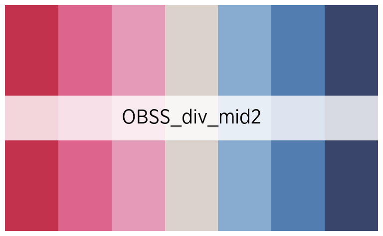

official_pal("OBSS_div_mid3", 7, show_pal = T)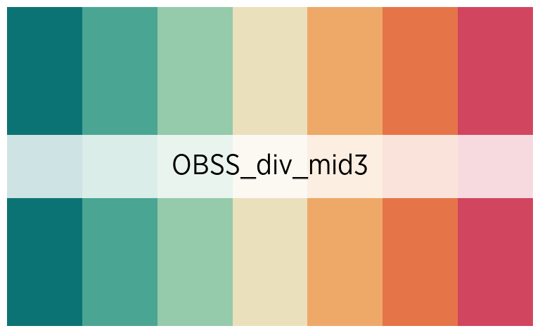

official_pal("OBSS_div_mid4", 7, show_pal = T)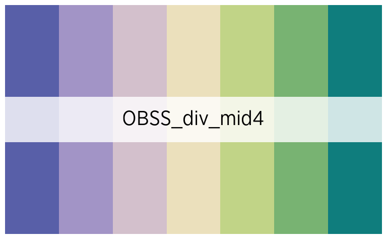

Sans point central

Attention, ces palettes ne sont symétriques que si le nombre de couleur est pair !

official_pal("OBSS_div_bi1", 8, show_pal = T)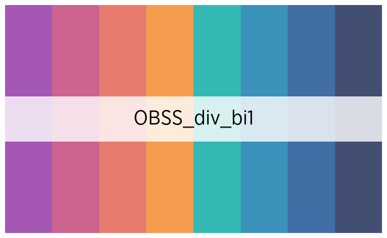

official_pal("OBSS_div_bi2", 8, show_pal = T)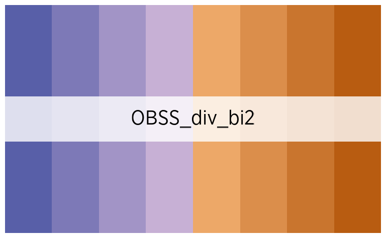

official_pal("OBSS_div_bi3", 8, show_pal = T)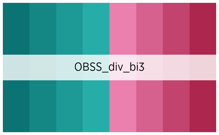

official_pal("OBSS_div_bi4", 8, show_pal = T)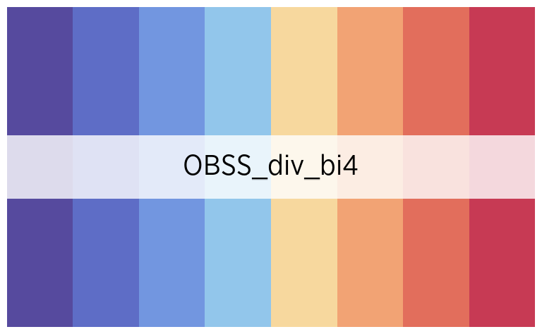

Palettes avec emphase

Il s’agit de palettes de couleur mettant en opposition la première, ou les deux premières catégories, avec toutes les autres :

official_pal("OBSS_highlight1", 8, show_pal = T)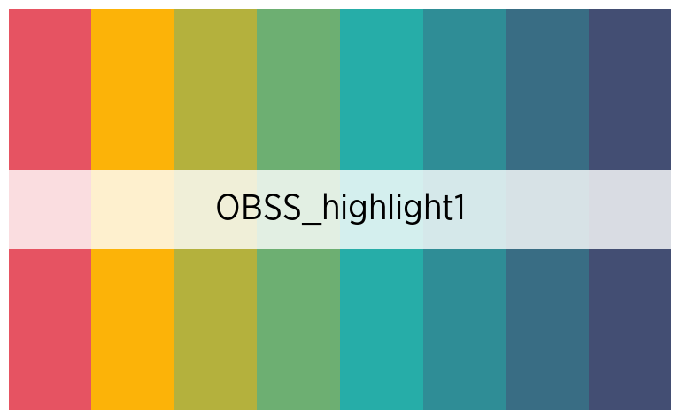

official_pal("OBSS_highlight2", 8, show_pal = T)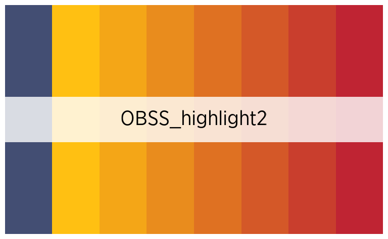

official_pal("OBSS_highlight3", 8, show_pal = T)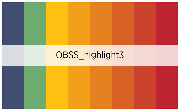

Palettes d’autres institutions

official_pal("IBSA", 4, show_pal = T)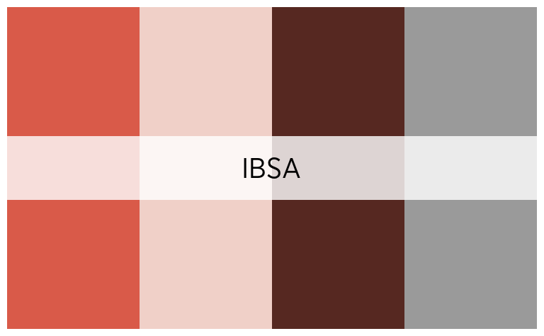

official_pal("ULB", 6, show_pal = T)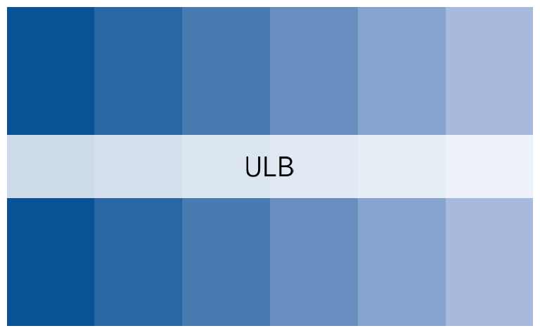

Altération des palettes

Il est possible de désaturer, éclaircir ou foncer les palettes, avec les arguments desaturate, lighten et darken, à la fois dans les fonctions de description de données de fonctionr et dans la fonction official_pal().

official_pal("OBSS", 8, show_pal = T)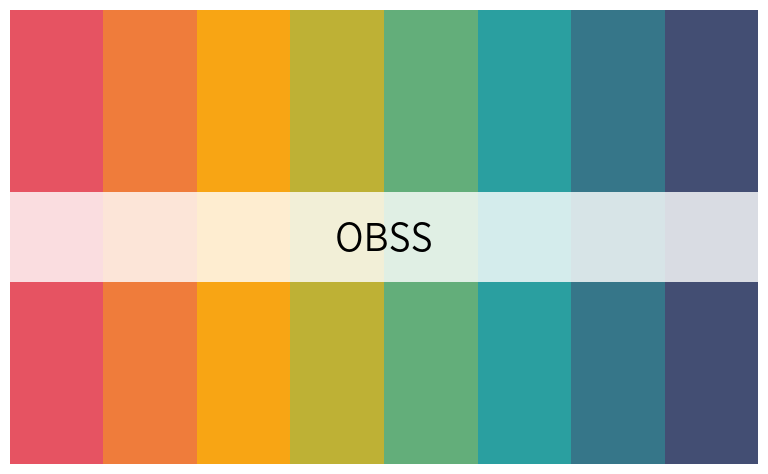

official_pal("OBSS", 8, desaturate = .4, show_pal = T)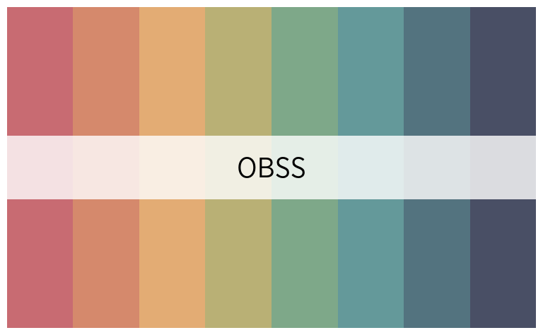

official_pal("OBSS", 8, lighten = .4, show_pal = T)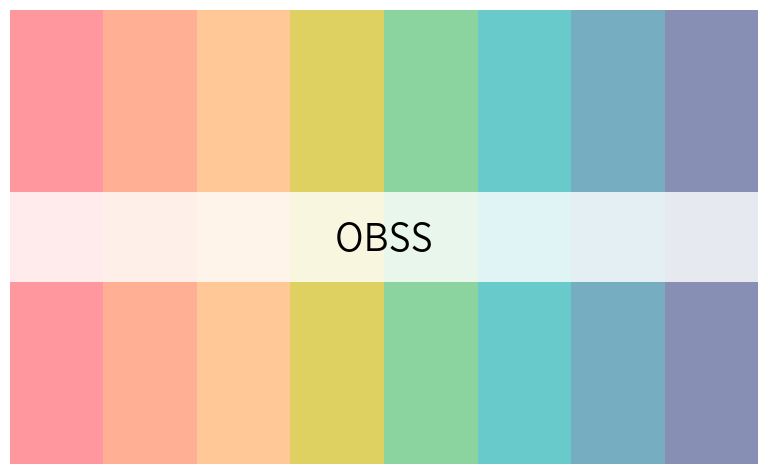

official_pal("OBSS", 8, darken = .4, show_pal = T)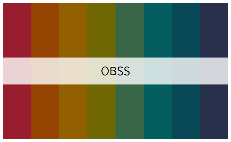

Exemples de graphiques

distrib_income_2 <- distrib_group_c(
  eusilc,
  db040,
  (py010n + py050n) / 12,
  filter_exp = pl030 == 2,
  limits = c(-500, 3000),
  show_mid_point = F,
  show_value = F,
  show_ci_errorbar = F,
  show_moustache = F,
  pal = official_pal(inst = "OBSS_Purples", n = 2, direction = -1),
  alpha = .8,
  font = "Gotham Narrow",
  title = "Income from wage, part time workers by region"
)

distrib_income_2$graph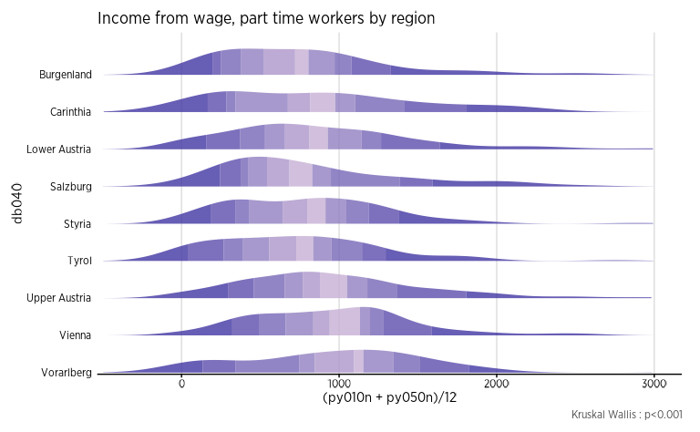

eusilc_dist_group_d <- distrib_group_d(
  eusilc,
  group = db040,
  quali_var = pl030_rec,
  filter_exp = age > 12,
  pal = "OBSS_alt1",
  font = "Gotham Narrow",
  title = "Distribution of socio-economic status according to region"
  )

eusilc_dist_group_d$graph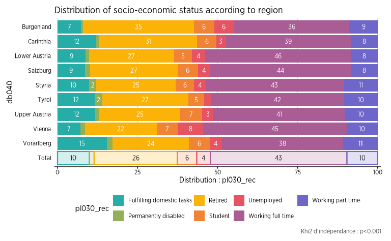

eusilc_many_mean_group <- many_mean_group(
  eusilc,
  group = rb090,
  list_vars = c(py010n, py050n, py090n),
  list_vars_lab = c("salaires", "revenus d'une activité indépendant", "allocation de chômage"),
  pal = "OBSS_Greens",
  unit = "€",
  font = "Gotham Narrow",
  title = "Income from wage, independant worker and unemployement benefits by sex"
  )

eusilc_many_mean_group$graph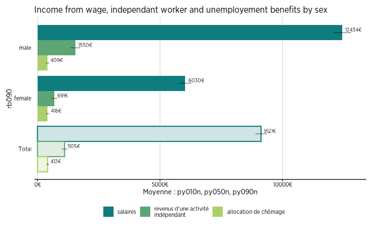

eusilc_dist_group_d2 <- distrib_group_d(
  eusilc,
  weights = rb050,
  group = pb220a,
  quali_var = pl030_rec,
  pal = "OBSS_Autumn",
  font = "Gotham Narrow",
  title = "Distribution of socio-economic status according to nationality"
  )

eusilc_dist_group_d2$graph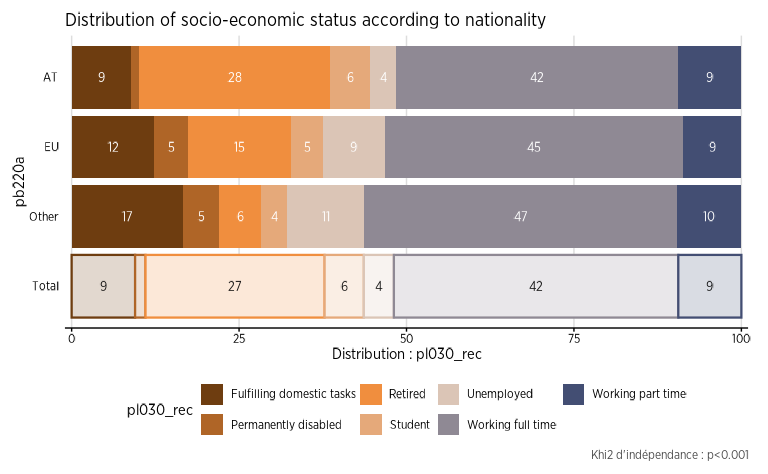

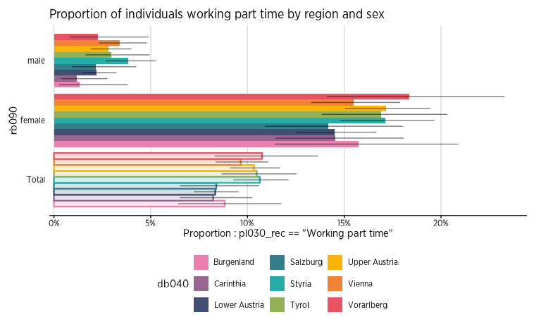
eusilc_prop_group <- prop_group(
  eusilc,
  group = rb090,
  prop_exp = pl030_rec == "Working part time",
  group.fill = db040,
  show_value = F,
  pal = "OBSS_alt2",
  font = "Gotham Narrow",
  title = "Proportion of individuals working part time by region and sex"
)

eusilc_prop_group$graph