Function to describe the distribution of a continuous variable from complex survey data. It produces a list containing a density table (dens), a central value table (tab), a quantile table (quant) and a ready-to-be published ggplot graphic (graph).
The density table contains x-y coordinates to draw a density curve. The central value table contains the median or the mean of the continuous variable, with its confidence interval, the sample size and the estimation of the total, with its confidence interval. The quantile table contains quantiles and their confidence intervals. The quantiles and the limits are used as thicks on the X axe of the graphic. The confidence intervals are taking into account the complex survey design.
Exporting those results to an Excell file is possible.
Usage
distrib_continuous(
  data,
  quanti_exp,
  type = "median",
  facet = NULL,
  filter_exp = NULL,
  ...,
  na.rm.facet = TRUE,
  quantiles = seq(0.1, 0.9, 0.1),
  bw = 1,
  resolution = 1024,
  limits = NULL,
  show_mid_line = TRUE,
  show_ci_lines = TRUE,
  show_ci_area = FALSE,
  show_quant_lines = FALSE,
  show_n = FALSE,
  show_value = TRUE,
  show_labs = TRUE,
  digits = 0,
  unit = "",
  dec = NULL,
  pal = NULL,
  col_density = c("#00708C", "mediumturquoise"),
  color = NULL,
  col_border = NA,
  font = "Roboto",
  title = NULL,
  subtitle = NULL,
  xlab = NULL,
  ylab = NULL,
  caption = NULL,
  lang = "fr",
  theme = "fonctionr",
  coef_font = 1,
  export_path = NULL
)

distrib_c(...)
Arguments
- data
A dataframe or an object from the survey package or an object from the srvyr package.
- quanti_exp
An expression defining the quantitatie variable the variable to be described. Notice that any observations with
NAin at least one of the variable inquanti_expare excluded for the computation of the density and of the indicators.- type
Type of central value :
"mean"to compute mean as the central value ;"median"to compute median as the central value.- facet
Not yet implemented.
- filter_exp
An expression filtering the data, preserving the design. Notice that
filter_expworks assrvyr::filter(): it excludes observations for whichfilter_expresults intoNA.It is often the case whenNAis present on one of the filter variables.- ...
All options possible in
srvyr::as_survey_design().- na.rm.facet
Not yet implemented.
- quantiles
Quantiles computed. Default are deciles.
- bw
The smoothing bandwidth to be used. The kernels are scaled such that this is the standard deviation of the smoothing kernel. Default is
1.- resolution
Resolution of the density curve. Default is
1024.- limits
Limits of the X axe of the graphic. Does not apply to the computation of indicators (median/mean and quantiles). Default is
NULLto show the entire distribution on the graphic.- show_mid_line
TRUEif you want to show the mean or median (depending on type) as a line on the graphic.FALSEif you do not want to show it. Default isTRUE.- show_ci_lines
TRUEif you want to show confidence interval of the mean or median (depending on type) as dotted lines on the graphic.FALSEif you do not want to show it as lines. Default isTRUE.- show_ci_area
TRUEif you want to show confidence interval of the mean or median (depending on type) as a coloured area on the graphic.FALSEif you do not want to show it as an area. Default isFALSE.- show_quant_lines
TRUEif you want to show quantiles as lines on the graphic.FALSEif you do not want to show them as lines. Default isFALSE.- show_n
TRUEif you want to show on the graphic the number of individuals in the sample in each quantile.FALSEif you do not want to show the numbers. Default isFALSE.- show_value
TRUEif you want to show the value of the mean/median (depending on type) on the graphic.FALSEif you do not want to show the mean/median. Default isTRUE.- show_labs
TRUEif you want to show axes labels.FALSEif you do not want to show any labels on axes. Default isTRUE.- digits
Number of decimal places displayed on the values labels on the graphic. Default is
0.- unit
Unit displayed on the graphic. Default is none (
"").- dec
Decimal mark shown on the graphic. Depends on lang:
","for fr and nl ;"."for en.- pal
For compatibility with older versions.
- col_density
Color of the density area. It may be one color or a vector with several colors. Colors should be R color or an hexadecimal color code. In case of one color, the density is monocolor. In case of a vector, the quantile areas are painted in continuous colors going from the last color in the vector (center quantile) to the first color (first and last quantiles). In case of an even quantile area numbers (e.g. deciles, quartiles) the last color of the vector is only applied to the highcenter quantile area to avoid two continuous quantile areas having the same color.
- color
Not currently used except for compatibility with old versions.
- col_border
Color of the density line. Color should be one R color or one hexadecimal color code. Default (
NULL) does not draw the density line.- font
Font used in the graphic. See
load_and_active_fonts()for available fonts. Default is"Roboto".- title
Title of the graphic.
- subtitle
Subtitle of the graphic.
- xlab
X label on the graphic. If
xlab = NULL, X label on the graphic will bequanti_exp.- ylab
Y label on the graphic. If
ylab = NULL, Y label on the graphic will be"Densité"(iflang = "fr"),"Density"(iflang = "en") or"Densiteit"(iflang = "nl").- caption
Caption of the graphic.
- lang
Language of the indications on the graphic. Possibilities are
"fr"(french),"nl"(dutch) and"en"(english). Default is"fr".- theme
Theme of the graphic. Default is
"fonctionr"."IWEPS"adds y axis lines and ticks.NULLuses the default grey ggplot2 theme.- coef_font
A multiplier factor for font size of all fonts on the graphic. Default is
1. Usefull when exporting the graphic for a publication (e.g. in a Quarto document).- export_path
Path to export the results in an xlsx file. The file includes four sheets: the central value table, the quantile table, the density table and the graphic.
Value
A list that contains a density table (dens), a central value table (tab), a quantile table (quant) and a ggplot graphic (graph).
Examples
# Loading of data
data(eusilc, package = "laeken")
# Computation, taking sample design into account
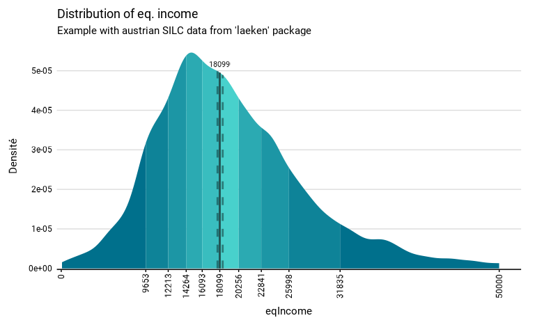
eusilc_dist_c <- distrib_c(
eusilc,
quanti_exp = eqIncome,
strata = db040,
ids = db030,
weight = rb050,
limits = c(0, 50000),
title = "Distribution of eq. income",
subtitle = "Example with austrian SILC data from 'laeken' package"
)
#> Input: data.frame
#> Sampling design -> ids: db030, strata: db040, weights: rb050
#> Variable(s) detected in quanti_exp: eqIncome
#> Numbers of observation(s) removed by each filter (one after the other):
#> 0 observation(s) removed due to missing value(s) for the variable(s) in quanti_exp
# Results in graph form
eusilc_dist_c$graph
#> Warning: Removed 701 rows containing missing values or values outside the scale range
#> (`geom_ribbon()`).
#> Warning: Removed 1042 rows containing missing values or values outside the scale range
#> (`geom_line()`).
 # Results in table format
eusilc_dist_c$tab
#> # A tibble: 1 × 7
#> median median_low median_upp n_sample n_weighted n_weighted_low n_weighted_upp
#> <dbl> <dbl> <dbl> <int> <dbl> <dbl> <dbl>
#> 1 18099. 17842. 18431. 14827 8182222 8079226. 8285218.
# Results in table format
eusilc_dist_c$tab
#> # A tibble: 1 × 7
#> median median_low median_upp n_sample n_weighted n_weighted_low n_weighted_upp
#> <dbl> <dbl> <dbl> <int> <dbl> <dbl> <dbl>
#> 1 18099. 17842. 18431. 14827 8182222 8079226. 8285218.