distrib_discrete

Function to describe the distribution of a discrete variable from complex survey data. It produces a list containing a table, including the confidence intervals of the indicators, a ready-to-be published ggplot graphic and, if proportions for H0 are specified, a Chi-Square statistical test (using survey::svygofchisq). Exporting those results to an Excell file is possible. The confidence intervals and the statistical test are taking into account the complex survey design. In case of facets, no statistical test is (yet) computed.

Usage

distrib_discrete(
  data,
  quali_var,
  facet = NULL,
  filter_exp = NULL,
  ...,
  na.rm.facet = TRUE,
  na.rm.var = TRUE,
  probs = NULL,
  prop_method = "beta",
  reorder = FALSE,
  show_ci = TRUE,
  show_n = FALSE,
  show_value = TRUE,
  show_labs = TRUE,
  scale = 100,
  digits = 0,
  unit = "%",
  dec = NULL,
  col = "sienna2",
  pal = NULL,
  dodge = 0.9,
  font = "Roboto",
  wrap_width_y = 25,
  title = NULL,
  subtitle = NULL,
  xlab = NULL,
  ylab = NULL,
  caption = NULL,
  lang = "fr",
  theme = "fonctionr",
  coef_font = 1,
  export_path = NULL
)

distrib_d(...)

Arguments

data

A dataframe or an object from the survey package or an object from the srvyr package.

quali_var

The discrete variable to be described.

facet

A variable defining the faceting group.

filter_exp

An expression filtering the data, preserving the design. Notice that filter_exp works as srvyr::filter() : it excludes observations for which filter_exp results into NA. It is often the case when NA is present on one of the filter variables.

...

All options possible in as_survey_design in srvyr package.

na.rm.facet

TRUE if you want to remove observations with NA on the facet variable. FALSE if you want to create a facet with the NA values for the facet variable. Default is TRUE.

na.rm.var

TRUE if you want to remove observations with NA on the discrete variable. FALSE if you want to create a modality with NA values for the discrete variable. Default is TRUE.

probs

Vector of probabilities for H0 of the statistical test, in the correct order (will be rescaled to sum to 1). If probs = NULL, no statistical test is performed. Default is NULL.

prop_method

Type of proportion method used to compute confidence intervals. See survey::svyciprop() for details. Default is beta method.

reorder

TRUE if you want to reorder the groups according to the proportion. NA value, in case if na.rm.var = FALSE, is not included in the reorder. In case of facets, the categories are reordered based on each median category Default is FALSE.

show_ci

TRUE if you want to show the error bars on the graphic. FALSE if you don't want to show the error bars. Default is TRUE.

show_n

TRUE if you want to show on the graphic the number of observations in the sample in each category. FALSE if you don't want to show this number. Default is FALSE.

show_value

TRUE if you want to show the proportions in each category on the graphic. FALSE if you don't want to show the proportion. Default is TRUE.

show_labs

TRUE if you want to show axes labels. FALSE if you do not want to show any label on axes. Default is TRUE.

scale

Denominator of the proportion. Default is 100 to interprets numbers as percentages.

digits

Number of decimal places displayed on the values labels on the graphic. Default is 0.

unit

Unit displayed on the graphic. Default is percent.

dec

Decimal mark displayed on the graphic. Default depends on lang: "," for fr and nl ; "." for en.

col

Color of the bars. col must be a R color or an hexadecimal color code. Default is "sienna2". The color of NA category (in case of na.rm.var == FALSE) is always "grey".

pal

Argument kept for compatibility with old versions.

dodge

Width of the bars. Default is 0.9 to let a small space between bars. A value of 1 leads to no space betweens bars. Values higher than 1 are not advised because they cause an overlaping of the bars.

font

Font used in the graphic. See load_and_active_fonts() for available fonts. Default is "Roboto".

wrap_width_y

Number of characters before going to the line for the labels of the categories. Default is 25.

title

Title of the graphic.

subtitle

Subtitle of the graphic.

xlab

X label on the graphic. As coord_flip() is used in the graphic, xlab refers to the x label on the graphic, after the coord_flip(), and not to the x variable in the data. Default (xlab = NULL) displays "Distribution (total : 100 pourcent)" (if lang == "fr"), "Distribution (total: 100 percent)" (if lang == "en" ) or "Distributie (totaal : 100 procent)" (if lang == "nl"). To show no X label, use xlab = "".

ylab

Y label on the graphic. As coord_flip() is used in the graphic, ylab refers to the Y label on the graphic, after the coord_flip(), and not to the Y variable in the data. Default (ylab = NULL) displays the name of the discrete variable (quali_var). To show no Y label, use ylab = "".

caption

Caption of the graphic. This caption goes under de default caption showing the result of the statistical test (if any).

lang

Language of the indications on the graphic. Possibilities are "fr" (french), "nl" (dutch) and "en" (english). Default is "fr".

theme

Theme of the graphic. Default is "fonctionr". "IWEPS" adds y axis lines and ticks. NULL uses the default grey ggplot2 theme.

coef_font

A multiplier factor for font size of all fonts on the graphic. Default is 1. Usefull when exporting the graphic for a publication (e.g. in a Quarto document).

export_path

Path to export the results in an xlsx file. The file includes two or three sheets : the table, the graphic and the statistical test (if probs is not NULL).

Value

A list that contains a table, a ggplot graphic and, if probs is not NULL, a statistical test.

Examples

# Loading of data
data(eusilc, package = "laeken")

# Recoding eusilc$pl030 into eusilc$pl030_rec
eusilc$pl030_rec <- NA
eusilc$pl030_rec[eusilc$pl030 == "1"] <- "Working full time"
eusilc$pl030_rec[eusilc$pl030 == "2"] <- "Working part time"
eusilc$pl030_rec[eusilc$pl030 == "3"] <- "Unemployed"
eusilc$pl030_rec[eusilc$pl030 == "4"] <- "Student"
eusilc$pl030_rec[eusilc$pl030 == "5"] <- "Retired"
eusilc$pl030_rec[eusilc$pl030 == "6"] <- "Permanently disabled"
eusilc$pl030_rec[eusilc$pl030 == "7"] <- "Fulfilling domestic tasks"

# Computation, taking sample design into account
eusilc_dist_group_d <- distrib_d(
eusilc,
pl030_rec,
strata = db040,
ids = db030,
weight = rb050,
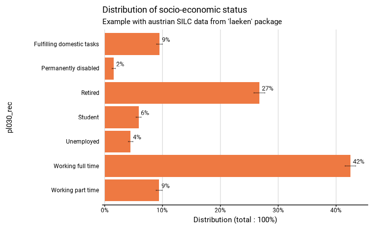
title = "Distribution of socio-economic status",
subtitle = "Example with austrian SILC data from 'laeken' package"
)
#> Input: data.frame
#> Sampling design -> ids:  db030, strata:  db040, weights:  rb050
#> Numbers of observation(s) removed by each filter (one after the other): 
#> 2720 observation(s) removed due to missing quali_var

# Results in graph form
eusilc_dist_group_d$graph


# Results in table format
eusilc_dist_group_d$tab
#> # A tibble: 7 × 8
#>   pl030_rec            prop prop_low prop_upp n_sample n_weighted n_weighted_low
#>   <fct>               <dbl>    <dbl>    <dbl>    <int>      <dbl>          <dbl>
#> 1 Fulfilling domest… 0.0948   0.0899   0.0998     1207    640311.        605978.
#> 2 Permanently disab… 0.0155   0.0129   0.0186      178    104930.         85796.
#> 3 Retired            0.267    0.258    0.277      3146   1806954.       1746273.
#> 4 Student            0.0586   0.0544   0.0630      736    395829.        365532.
#> 5 Unemployed         0.0449   0.0411   0.0489      518    303252.        276953.
#> 6 Working full time  0.425    0.416    0.434      5162   2869868.       2797833.
#> 7 Working part time  0.0941   0.0890   0.0995     1160    636121.        600709.
#> # ℹ 1 more variable: n_weighted_upp <dbl>