distrib_group_continuous — distrib_group

Function to compare the distribution of a continuous variable between groups from complex survey data. It produces a list containing a density table (dens), a central value table (tab), a quantile table (quant), a ready-to-be published ggplot graphic (graph), a box-plot table (moustache) and a statistical test (test). The density table contains x-y coordinates to draw density curve for each group. The central value table contains, for each group, the median or the mean of the continuous variable, with their confidence intervals, the sample size and the estimations of the totals, with their confidence intervals. The quantile table contains, for each group, quantiles and their confidence intervals. The box-plot table contains the X coordinates to draw the moustache, for each group. In case of mean comparison, the statistical test is a Wald test (using survey::regTermTest). In case of median comparison the statistical test is a Kruskal Wallis test (using survey::svyranktest(test = "KruskalWallis")). Exporting those results to an Excell file is possible. The confidence intervals are taking into account the complex survey design.

Usage

distrib_group_continuous(
  data,
  group,
  quanti_exp,
  type = "median",
  facet = NULL,
  filter_exp = NULL,
  ...,
  na.rm.group = TRUE,
  na.rm.facet = TRUE,
  quantiles = seq(0.1, 0.9, 0.1),
  moustache_probs = c(0.95, 0.8, 0.5),
  bw = 1,
  resolution = 512,
  height = 0.8,
  limits = NULL,
  reorder = FALSE,
  show_mid_point = TRUE,
  show_mid_line = FALSE,
  show_ci_errorbar = TRUE,
  show_ci_lines = FALSE,
  show_ci_area = FALSE,
  show_quant_lines = FALSE,
  show_moustache = TRUE,
  show_value = TRUE,
  show_labs = TRUE,
  digits = 0,
  unit = "",
  dec = NULL,
  pal = NULL,
  col_density = "#e0dfe0",
  pal_moustache = NULL,
  col_moustache = c("#EB9BA0", "#FAD7B1"),
  color = NULL,
  col_border = NA,
  alpha = 1,
  font = "Roboto",
  wrap_width_y = 25,
  title = NULL,
  subtitle = NULL,
  xlab = NULL,
  ylab = NULL,
  caption = NULL,
  lang = "fr",
  theme = "fonctionr",
  coef_font = 1,
  export_path = NULL
)

distrib_group_c(...)

Arguments

data: A dataframe or an object from the survey package or an object from the srvyr package.
group: A variable defining groups to be compared.
quanti_exp: An expression defining the quantitatie variable the variable to be described and compared between groups. Notice that any observations with NA in at least one of the variable in quanti_exp are excluded for the computation of the densities and of the indicators.
type: Type of central value : "mean" to compute mean as the central value by group ; "median" to compute median as the central value by group.
facet: Not yet implemented.
filter_exp: An expression filtering the data, preserving the design. Notice that filter_exp works as srvyr::filter() : it excludes observations for which filter_exp results into NA. It is often the case when NA is present on one of the filter variables.
...: All options possible in as_survey_design in srvyr package.
na.rm.group: TRUE if you want to remove observations with NA on the group variable. FALSE if you want to create a group with the NA values for the group variable. Default is TRUE.
na.rm.facet: Not yet implemented.
quantiles: Quantiles computed in the distributions. Default are deciles.
moustache_probs: A vector defining the proportions of the population used to draw the boxplot. Default is 0.95, 0.8, 0.5 to draw a boxplot with three groups containing respectively 50 percent, 80 percent and 95 percent of the population around to the median.
bw: The smoothing bandwidth to be used. The kernels are scaled such that this is the standard deviation of the smoothing kernel. Default is 1.
resolution: Resolution of the density curve. Default is 512
height: Height of the curves. Default is 0.8. Values higher than 1 may cause curves to overlap.
limits: Limits of the x axe of the graphic. Does not apply to the computation. Default is NULL to show the entire distribution on the graphic. If the limits are shorter than the boxplot, some part of some boxplot will not be drawn.
reorder: TRUE if you want to reorder the groups according to the mean/median (depending on type). Unlike other functions, NA values, in case if na.rm.group = FALSE, is included in the reorder.
show_mid_point: TRUE if you want to show the mean or median (depending on type) as a point on the graphic. FALSE if you do not want to. Default is TRUE.
show_mid_line: TRUE if you want to show the mean or median (depending on type) as a line on the graphic. FALSE if you do not want to. Default is FALSE
show_ci_errorbar: TRUE if you want to show confidence interval of the mean or median (depending on type) as an error bar on the graphic. FALSE if you do not want to show it as lines. Default is TRUE.
show_ci_lines: TRUE if you want to show confidence interval of the mean or median (depending on type) as lines on the graphic. FALSE if you do not want to show it as lines. Default is FALSE
show_ci_area: TRUE if you want to show confidence interval of the mean or median (depending on type) as a coloured area on the graphic. FALSE if you do not want to show it as an area. Default is FALSE.
show_quant_lines: TRUE if you want to show quantiles as lines on the graphic. FALSE if you do not want to show them as lines. Default is FALSE.
show_moustache: TRUE if you want to show the boxplot on the graphic. FALSE if you do not want to show it. Default is TRUE.
show_value: TRUE if you want to show the value of mean/median of each group on the graphic. FALSE if you do not want to show the mean/median. Default is TRUE.
show_labs: TRUE if you want to show axes labels. FALSE if you do not want to show any labels on axes. Default is TRUE.
digits: Number of decimal places displayed on the values labels on the graphic. Default is 0.
unit: Unit displayed on the graphic. Default is none.
dec: Decimal mark shown on the graphic. Depends on lang: "," for fr and nl ; "." for en.
pal: For compatibility with older versions.
col_density: Color of the density area. It may be one color or a vector with several colors. Colors should be R color or an hexadecimal color code. In case of one color, the density is monocolor. In case of a vector, the quantile areas are painted in continuous colors going from the last color in the vector (center quantile) to the first color (first and last quantiles). In case of an even quantile area numbers (e.g. deciles, quartiles) the last color of the vector is only applied to the highcenter quantile area to avoid two continuous quantile areas having the same color.
pal_moustache: For compatibility with old versions.
col_moustache: Color of the moustache. Can be one or several colors to create a palette. In case of a vector, the different areas of the box-plot are painted in continuous colors going from the first color in the vector (center of the bo-plot) to the last color (extern area of the box-plot).
color: For compatibility with older versions.
col_border: Color of the density line. Color should be one R color or one hexadecimal color code. Default (NULL) does not draw the density line.
alpha: Transparence of the density areas. Default is 1. It applies only to col_density.
font: Font used in the graphic. See load_and_active_fonts() for available fonts. Default is "Roboto".
wrap_width_y: Number of characters before going to the line for the labels of the groups. Default is 25.
title: Title of the graphic.
subtitle: Subtitle of the graphic.
xlab: X label on the graphic. As coord_flip() is used in the graphic, xlab refers to the X label on the graphic, after the coord_flip(), and not to the x variable in the data. If xlab = NULL, X label on the graphic will be quanti_exp.
ylab: Y label on the graphic. As coord_flip() is used in the graphic, ylab refers to the y label on the graphic, after the coord_flip(), and not to the y variable in the data. Default (ylab = NULL) displays the name of the group variable. To show no Y label, use ylab = "".
caption: Caption of the graphic. This caption goes under de default caption showing the result of the Chi-Square test. There is no way of not showing the result of the statistical test as a caption.
lang: Language of the indications on the graphic. Possibilities are "fr" (french), "nl" (dutch) and "en" (english). Default is "fr".
theme: Theme of the graphic. Default is "fonctionr". "IWEPS" adds y axis lines and ticks. NULL uses the default grey ggplot2 theme.
coef_font: A multiplier factor for font size of all fonts on the graphic. Default is 1. Usefull when exporting the graphic for a publication (e.g. in a Quarto document).
export_path: Path to export the results in an xlsx file. The file includes five sheets: the central values table, the quantile table, the densities table, the graphic and the statistical test result.

Value

A list that contains a density table (dens), a central values table (tab), a quantile table (quant), a ggplot graphic (graph), boxplot table (moustache) and a statistical test (test).

Examples

# Loading of data
data(eusilc, package = "laeken")

# Recoding eusilc$pl030 into eusilc$pl030_rec
eusilc$pl030_rec <- NA
eusilc$pl030_rec[eusilc$pl030 == "1"] <- "Working full time"
eusilc$pl030_rec[eusilc$pl030 == "2"] <- "Working part time"
eusilc$pl030_rec[eusilc$pl030 == "3"] <- "Unemployed"
eusilc$pl030_rec[eusilc$pl030 == "4"] <- "Student"
eusilc$pl030_rec[eusilc$pl030 == "5"] <- "Retired"
eusilc$pl030_rec[eusilc$pl030 == "6"] <- "Permanently disabled"
eusilc$pl030_rec[eusilc$pl030 == "7"] <- "Fulfilling domestic tasks"

# Computation, taking sample design into account
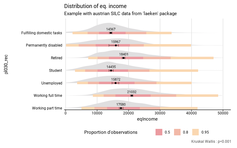
eusilc_dist_g_c <- distrib_group_c(
  eusilc,
  group = pl030_rec,
  quanti_exp = eqIncome,
  strata = db040,
  ids = db030,
  weight = rb050,
  limits = c(0, 50000),
  resolution = 128,
  title = "Distribution of eq. income",
  subtitle = "Example with austrian SILC data from 'laeken' package"
)
#> Input: data.frame
#> Sampling design -> ids:  db030, strata:  db040, weights:  rb050
#> Variable(s) detected in quanti_exp: eqIncome
#> Numbers of observation(s) removed by each filter (one after the other): 
#> 2720 observation(s) removed due to missing group
#> 0 observation(s) removed due to missing value(s) for the variable(s) in quanti_exp

# Results in graph form
eusilc_dist_g_c$graph
#> Warning: Removed 497 rows containing missing values or values outside the scale range
#> (`geom_ribbon()`).
#> Warning: Removed 1022 rows containing missing values or values outside the scale range
#> (`geom_line()`).


# Results in table format
eusilc_dist_g_c$tab
#> # A tibble: 7 × 8
#>   pl030_rec      median median_low median_upp n_sample n_weighted n_weighted_low
#>   <chr>           <dbl>      <dbl>      <dbl>    <int>      <dbl>          <dbl>
#> 1 Fulfilling do… 14367.     13918.     14774.     1207    640311.        605978.
#> 2 Permanently d… 15967.     13753.     16797.      178    104930.         85796.
#> 3 Retired        18401.     17956.     18887.     3146   1806954.       1746273.
#> 4 Student        14435.     13780.     15133.      736    395829.        365532.
#> 5 Unemployed     15872.     14725.     16900.      518    303252.        276953.
#> 6 Working full … 21032.     20644.     21406.     5162   2869868.       2797833.
#> 7 Working part … 17580.     17043.     18270.     1160    636121.        600709.
#> # ℹ 1 more variable: n_weighted_upp <dbl>