distrib_group_discrete

Function to compare the distribution of a discrete variable between different groups based on complex survey data. It produces a list containing a table, including the confidence intervals of the indicators, a ready-to-be published ggplot graphic and a Chi-Square statistical test (using survey::svychisq). Exporting those results to an Excell file is possible. The confidence intervals and the statistical test are taking into account the complex survey design. In case of facets, no statistical test is (yet) computed.

Usage

distrib_group_discrete(
  data,
  group,
  quali_var,
  facet = NULL,
  filter_exp = NULL,
  ...,
  na.rm.group = T,
  na.rm.facet = T,
  na.rm.var = T,
  total = TRUE,
  prop_method = "beta",
  reorder = F,
  show_n = FALSE,
  show_value = TRUE,
  show_labs = TRUE,
  total_name = NULL,
  scale = 100,
  digits = 0,
  unit = "",
  dec = NULL,
  pal = "OBSS",
  direction = 1,
  desaturate = 0,
  lighten = 0,
  darken = 0,
  dodge = 0.9,
  font = "Roboto",
  wrap_width_y = 25,
  wrap_width_leg = 25,
  legend_ncol = 4,
  title = NULL,
  subtitle = NULL,
  xlab = NULL,
  ylab = NULL,
  legend_lab = NULL,
  caption = NULL,
  lang = "fr",
  theme = "fonctionr",
  coef_font = 1,
  export_path = NULL
)

distrib_group_d(...)

Arguments

data

A dataframe or an object from the survey package or an object from the srvyr package.

group

A variable defining groups to be compared.

quali_var

The discrete variable described among the different groups.

facet

A variable defining the faceting group.

filter_exp

An expression filtering the data, preserving the design. Notice that filter_exp works as srvyr::filter() : it excludes observations for which filter_exp results into NA. It is often the case when NA is present on one of the filter variables.

...

All options possible in as_survey_design in srvyr package.

na.rm.group

TRUE if you want to remove observations with NA on the group. FALSE if you want to create a group with the NA values for the group variable. Default is TRUE.

na.rm.facet

TRUE if you want to remove observations with NA on the facet variable. FALSE if you want to create a facet with the NA values for the facet variable. Default is TRUE.

na.rm.var

TRUE if you want to remove observations with NA on the discrete variable. FALSE if you want to create a modality with NA values for the discrete variable. Default is TRUE.

total

TRUE if you want to compute a total, FALSE if you don't. The default is TRUE.

prop_method

Type of proportion method used to compute confidence intervals. See survey::svyciprop() for details. Default is beta method.

reorder

TRUE if you want to reorder the groups according to the proportion of the first level of quali_var. NA group, in case if na.rm.group = FALSE, is not included in the reorder. In case of facets, the groups are reordered based on each median group. Default is FALSE.

show_n

TRUE if you want to show on the graphic the number of observations in the sample in each category (of quali_var) of each group. FALSE if you don't want to show this number. Default is FALSE.

show_value

TRUE if you want to show the proportion in each category of each group on the graphic. FALSE if you do not want to show the proportions. Proportions of 2 percent or less are never showed on the graphic. Default is TRUE.

show_labs

TRUE if you want to show axes and legend labels. FALSE if you don't want to show any labels on axes and legend. Default is TRUE.

total_name

Name of the total displayed on the graphic. Default is "Total" in French and in English and "Totaal" in Dutch.

scale

Denominator of the proportions. Default is 100 to interpret numbers as percentages.

digits

Number of decimal places displayed on the values labels on the graphic. Default is 0.

unit

Unit showed in the graphic. Default (unit = "") shows not unit on values and percent on the X axe.

dec

Decimal mark shown on the graphic. Depends on lang: "," for fr and nl ; "." for en.

pal

Colors of the bars. pal must be vector of R colors or hexadecimal colors or a palette from packages MetBrewer or PrettyCols or a palette from fonctionr. The color of NA category (in case of na.rm.var == FALSE) is always "grey".

direction

Direction of the palette color. Default is 1. The opposite direction is -1.

desaturate

Numeric specifying the amount of desaturation where 1 corresponds to complete desaturation (no colors, grey layers only), 0 to no desaturation, and values in between to partial desaturation. Default is 0. See colorspace::desaturate for details. If desaturate and lighten/darken arguments are used, lighten/darken is applied in a second time (i.e. on the color transformed by desaturate).

lighten

Numeric specifying the amount of lightening. Negative numbers cause darkening. Value shoud be ranged between -1 (black) and 1 (white). Default is 0. It doesn't affect the color of NAs (in case of na.rm.group = FALSE). See colorspace::lighten for details. If both argument ligthen and darken are used (not advised), darken is applied in a second time (i.e. on the color transformed by lighten).

darken

Numeric specifying the amount of lightening. Negative numbers cause lightening. Value shoud be ranged between -1 (white) and 1 (black). Default is 0. It doesn't affect the color of NAs (in case of na.rm.group = FALSE). See colorspace::darken for details. If both argument ligthen and darken are used (not advised), darken is applied in a second time (i.e. on the color transformed by lighten).#'

dodge

Width of the bars. Default is 0.9 to let a small space between bars. A value of 1 leads to no space betweens bars. Values higher than 1 are not advised because they cause an overlaping of the bars.

font

Font used in the graphic. See load_and_active_fonts() for available fonts. Default is "Roboto".

wrap_width_y

Number of characters before going to the line for the labels of the groups. Default is 25.

wrap_width_leg

Number of characters before going to the line for the labels of quali_var. Default is 25.

legend_ncol

Number of columns in the legend. Default is 4.

title

Title of the graphic.

subtitle

Subtitle of the graphic.

xlab

X label on the graphic. As coord_flip() is used in the graphic, xlab refers to the x label on the graphic, after the coord_flip(), and not to the x variable in the data. Default (xlab = NULL) displays "Distribution : " (if lang == "fr"), "Distribution: " (if lang == "en" ) or "Distributie: " (if lang == "nl"), followed by the name of the discrete variable (quali_var). To show no X label, use xlab = "".

ylab

Y label on the graphic. As coord_flip() is used in the graphic, ylab refers to the y label on the graphic, after the coord_flip(), and not to the y variable in the data. Default (ylab = NULL) displays the name of the group variable. To show no Y label, use ylab = "".

legend_lab

Legend (fill) label on the graphic. Default (legend_lab = NULL) displays the name of the discrete variable (quali_var). To show no legend label, use legend_lab = "".

caption

Caption of the graphic. This caption goes under de default caption showing the result of the Chi-Square test. There is no way of not showing the result of the chi-square test as a caption.

lang

Language of the indications on the graphic. Possibilities are "fr" (french), "nl" (dutch) and "en" (english). Default is "fr".

theme

Theme of the graphic. Default is "fonctionr". "IWEPS" adds y axis lines and ticks. NULL uses the default grey ggplot2 theme.

coef_font

A multiplier factor for font size of all fonts on the graphic. Default is 1. Usefull when exporting the graphic for a publication (e.g. in a Quarto document).

export_path

Path to export the results in an xlsx file. The file includes three (without facets) or two sheets (with facets): the table, the graphic and the Chi-Square statistical test result.

Value

A list that contains a table, a ggplot graphic and, in most cases, a Chi-square statistical test.

Examples

# Loading of data
data(eusilc, package = "laeken")

# Recoding eusilc$pl030 into eusilc$pl030_rec
eusilc$pl030_rec <- NA
eusilc$pl030_rec[eusilc$pl030 == "1"] <- "Working full time"
eusilc$pl030_rec[eusilc$pl030 == "2"] <- "Working part time"
eusilc$pl030_rec[eusilc$pl030 == "3"] <- "Unemployed"
eusilc$pl030_rec[eusilc$pl030 == "4"] <- "Student"
eusilc$pl030_rec[eusilc$pl030 == "5"] <- "Retired"
eusilc$pl030_rec[eusilc$pl030 == "6"] <- "Permanently disabled"
eusilc$pl030_rec[eusilc$pl030 == "7"] <- "Fulfilling domestic tasks"

# Computation, taking sample design into account
eusilc_dist_d <- distrib_group_d(
eusilc,
group = pb220a,
quali_var = pl030_rec,
strata = db040,
ids = db030,
weight = rb050,
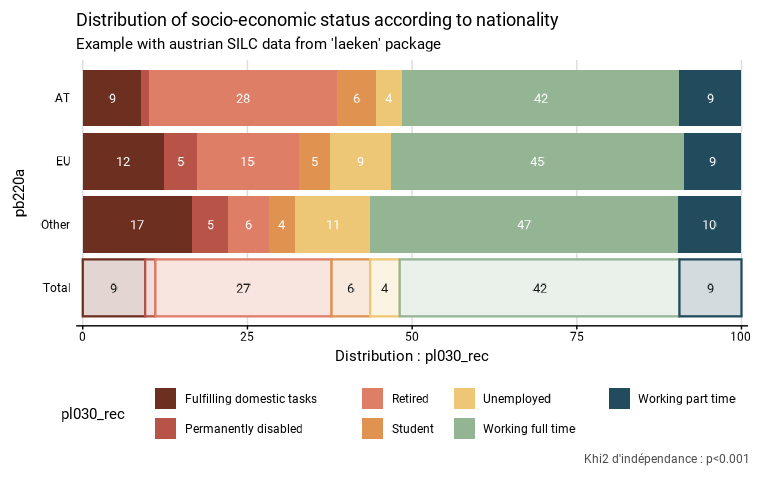
title = "Distribution of socio-economic status according to nationality",
subtitle = "Example with austrian SILC data from 'laeken' package"
)
#> Input: data.frame
#> Sampling design -> ids:  db030, strata:  db040, weights:  rb050
#> Numbers of observation(s) removed by each filter (one after the other): 
#> 2720 observation(s) removed due to missing group
#> 0 observation(s) removed due to missing quali_var

# Results in graph form
eusilc_dist_d$graph
#> Warning: Removed 21 rows containing missing values or values outside the scale range
#> (`geom_bar()`).
#> Warning: Removed 22 rows containing missing values or values outside the scale range
#> (`geom_text()`).
#> Warning: Removed 8 rows containing missing values or values outside the scale range
#> (`geom_text()`).


# Results in table format
eusilc_dist_d$tab
#> # A tibble: 28 × 9
#>    pb220a pl030_rec    prop prop_low prop_upp n_sample n_weighted n_weighted_low
#>    <fct>  <fct>       <dbl>    <dbl>    <dbl>    <int>      <dbl>          <dbl>
#>  1 AT     Fulfillin… 0.0890  0.0840    0.0942     1036    548489.        516433.
#>  2 AT     Permanent… 0.0119  0.00931   0.0150      125     73270.         56226.
#>  3 AT     Retired    0.285   0.275     0.295      3055   1754654.       1694827.
#>  4 AT     Student    0.0602  0.0558    0.0650      693    371222.        341944.
#>  5 AT     Unemployed 0.0388  0.0351    0.0427      411    238841.        215788.
#>  6 AT     Working f… 0.421   0.412     0.431      4689   2595137.       2526927.
#>  7 AT     Working p… 0.0942  0.0889    0.0998     1064    580514.        546750.
#>  8 EU     Fulfillin… 0.124   0.0886    0.167        38     20343.         13863.
#>  9 EU     Permanent… 0.0498  0.0280    0.0810       15      8186.          4024.
#> 10 EU     Retired    0.155   0.115     0.202        45     25429.         17953.
#> # ℹ 18 more rows
#> # ℹ 1 more variable: n_weighted_upp <dbl>