many_val — many_val • fonctionr

Function to compute the proportions of a set of several binary variables or means or medians of a set of quantitative variables, based on complex survey data.

It produces a list containing a table, including the confidence intervals of the indicators and a ready-to-be published ggplot graphic. The confidence intervals are taking into account the complex survey design.

Exporting the results to an Excell file is possible.

Usage

many_val(
  data,
  list_vars,
  type,
  list_vars_lab = NULL,
  facet = NULL,
  filter_exp = NULL,
  ...,
  na.rm.facet = TRUE,
  na.vars = "rm",
  prop_method = "beta",
  reorder = FALSE,
  show_ci = TRUE,
  show_n = FALSE,
  show_value = TRUE,
  show_labs = TRUE,
  scale = NULL,
  digits = 0,
  unit = NULL,
  dec = NULL,
  col = NULL,
  pal = "OBSS_alt3",
  direction = 1,
  desaturate = 0,
  lighten = 0,
  darken = 0,
  dodge = 0.9,
  font = "Roboto",
  wrap_width_y = 25,
  title = NULL,
  subtitle = NULL,
  xlab = NULL,
  ylab = NULL,
  caption = NULL,
  lang = "fr",
  theme = "fonctionr",
  coef_font = 1,
  export_path = NULL
)

many_prop(..., type = "prop")

many_median(..., type = "median")

many_mean(..., type = "mean")

Arguments

data: A dataframe or an object from the survey package or an object from the srvyr package.
list_vars: A vector containing the names of the dummy/quantitative variables on which to compute the proportions/means/medians.
type: "prop" to compute proportions ; "mean" to compute means ; "median" to compute medians.
list_vars_lab: A vector containing the labels of the dummy/quantitative variables to be displayed on the graphic and in the table of result. Default uses the variable names in list_vars.
facet: A variable defining the faceting group.
filter_exp: An expression filtering the data, preserving the design. Notice that filter_exp works as srvyr::filter(): it excludes observations for which filter_exp results into NA. It is often the case when NA is present on one of the filter variables.
...: All options possible in srvyr::as_survey_design().
na.rm.facet: TRUE if you want to remove observations with NA on the facet variable. FALSE if you want to create a facet with the NA values for the facet variable. Default is TRUE.
na.vars: The treatment of NA values in variables (list_vars). "rm" removes NA seperately in each individual variable, "rm.all" removes every individual that has at least one NA in one variable. Default is "rm".
prop_method: Type of proportion method used to compute confidence intervals. See survey::svyciprop() for details. Default is beta method. This argument is only used in case of type = "prop".
reorder: TRUE if you want to reorder the variables according to the proportions/means/medians. Default is FALSE.
show_ci: TRUE if you want to show the error bars on the graphic. FALSE if you don't want to show the error bars. Default is TRUE.
show_n: TRUE if you want to show on the graphic the number of observations in the sample for each variable. The number can varie if na.vars = "rm". FALSE if you do not want to show this number. Default is FALSE.
show_value: TRUE if you want to show the proportions/means/median for each variable on the graphic. FALSE if you do not want to show the proportions/means/medians. Default is TRUE.
show_labs: TRUE if you want to show axes labels. FALSE if you do not want to show any labels on axes. Default is TRUE.
scale: Denominator of the proportions. Default is 100 to interpret numbers as percentages. This argument is only used in case of type = "prop".
digits: Number of decimal places displayed on the values labels on the graphic. Default is 0.
unit: Unit displayed on the graphic. Default is percent for type = "prop" and no unit for type = "mean" or "median".
dec: Decimal mark displayed on the graphic. Default depends on lang: "," for fr and nl ; "." for en.
col: Color of the bars if the user wants a monocolor graph. col must be a R color or an hexadecimal color code. As pal has a priority over col, if the user wants to use col, he must not use simultaneously the pal argument (even pal = NULL).
pal: Colors of the bars if the user wants the bars to have different colors. pal must be vector of R colors or hexadecimal colors or a palette from packages MetBrewer or PrettyCols or a palette from fonctionr. pal has a priority over col.
direction: Direction of the palette color. Default is 1. The opposite direction is -1.
desaturate: Numeric specifying the amount of desaturation where 1 corresponds to complete desaturation (no colors, grey layers only), 0 to no desaturation, and values in between to partial desaturation. Default is 0. It affects only the palette (pal) and not the monocolor (col). See colorspace::desaturate() for details. If desaturate and lighten/darken arguments are used, lighten/darken is applied in a second time (i.e. on the color transformed by desaturate).
lighten: Numeric specifying the amount of lightening. Negative numbers cause darkening. Value shoud be ranged between -1 (black) and 1 (white). Default is 0. It affects only the palette (pal) and not the monocolor (col). See colorspace::lighten() for details. If both argument ligthen and darken are used (not advised), darken is applied in a second time (i.e. on the color transformed by lighten).
darken: Numeric specifying the amount of lightening. Negative numbers cause lightening. Value shoud be ranged between -1 (white) and 1 (black). Default is 0. It affects only the palette (pal) and not the monocolor (col). See colorspace::darken() for details. If both argument ligthen and darken are used (not advised), darken is applied in a second time (i.e. on the color transformed by lighten).
dodge: Width of the bars. Default is 0.9 to let a small space between bars. A value of 1 leads to no space betweens bars. Values higher than 1 are not advised because they cause an overlaping of the bars.
font: Font used in the graphic. See load_and_active_fonts() for available fonts. Default is "Roboto".
wrap_width_y: Number of characters before going to the line for the labels of the groups. Default is 25.
title: Title of the graphic.
subtitle: Subtitle of the graphic.
xlab: X label on the graphic. As ggplot2::coord_flip() is used in the graphic, xlab refers to the x label on the graphic, after the ggplot2::coord_flip(), and not to the x variable in the data. Default (xlab = NULL) displays, for type = prop, "Proportion :" (if lang = "fr"), "Proportion:" (if lang = "en") or "Aandeel:" (if lang = "nl"), or, for type = "mean", "Moyenne :" (if lang = "fr"), "Mean:" (if lang = "en") or "Gemiddelde:" (if lang = "nl"), or, for type = "median", "Médiane :" (if lang = "fr"), "Median:" (if lang = "en") or "Mediaan:" (if lang = "nl"), followed by the labels of the variables (list_vars_lab). To show no X label, use xlab = "".
ylab: Y label on the graphic. As ggplot2::coord_flip() is used in the graphic, ylab refers to the y label on the graphic, after the ggplot2::coord_flip(), and not to the y variable in the data. Default (ylab = NULL) displays no Y label.
caption: Caption of the graphic.
lang: Language of the indications on the graphic. Possibilities are "fr" (french), "nl" (dutch) and "en" (english). Default is "fr".
theme: Theme of the graphic. Default is "fonctionr". "IWEPS" adds y axis lines and ticks. NULL uses the default grey ggplot2 theme.
coef_font: A multiplier factor for font size of all fonts on the graphic. Default is 1. Usefull when exporting the graphic for a publication (e.g. in a Quarto document).
export_path: Path to export the results in an xlsx file. The file includes two sheets: the table and the graphic.

Value

A list that contains a table and a ggplot graphic.

Examples

# Loading of data
data(eusilc, package = "laeken")

# Recoding variables
eusilc$worker <- 0
eusilc$worker[eusilc$pl030 == "1"]<-1
eusilc$worker[eusilc$pl030 == "2"]<-1
eusilc$austrian<-0
eusilc$austrian[eusilc$pb220a == "AT"]<-1

# Computation, taking sample design into account
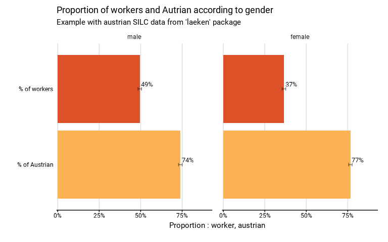
eusilc_many_prop <- many_prop(
  eusilc,
  list_vars = c(worker,austrian),
  list_vars_lab = c("% of workers","% of Austrian"),
  facet = rb090,
  strata = db040,
  ids = db030,
  weight = rb050,
  title = "Proportion of workers and Autrian according to gender",
  subtitle = "Example with austrian SILC data from 'laeken' package"
)
#> Variables used: worker, austrian
#> Input: data.frame
#> Sampling design -> ids:  db030, strata:  db040, weights:  rb050
#> Numbers of observation(s) removed by each filter (one after the other): 
#> 0 observation(s) removed due to missing facet
#> Warning: With na.vars = 'rm', observations removed differ between variables

# Results in graph form
eusilc_many_prop$graph


# Results in table format
eusilc_many_prop$tab
#> # A tibble: 4 × 12
#>   rb090  list_col       prop prop_low prop_upp n_sample n_true_weighted
#>   <fct>  <fct>         <dbl>    <dbl>    <dbl>    <int>           <dbl>
#> 1 male   % of workers  0.495    0.484    0.506     7267        1969092.
#> 2 female % of workers  0.366    0.355    0.376     7560        1536897.
#> 3 male   % of Austrian 0.739    0.728    0.750     7267        2942211.
#> 4 female % of Austrian 0.766    0.756    0.777     7560        3219916.
#> # ℹ 5 more variables: n_true_weighted_low <dbl>, n_true_weighted_upp <dbl>,
#> #   n_tot_weighted <dbl>, n_tot_weighted_low <dbl>, n_tot_weighted_upp <dbl>