Function to compare de proportions/means/medians of a set of several binary/quantitatives variables between different groups, based on complex survey data. It produces a list containing a table, including the confidence intervals of the indicators and a ready-to-be published ggplot graphic. The confidence intervals are taking into account the complex survey design.
Exporting the results to an Excell file is possible.
Usage
many_val_group(
  data,
  group,
  list_vars,
  type,
  list_vars_lab = NULL,
  facet = NULL,
  filter_exp = NULL,
  ...,
  na.rm.group = TRUE,
  na.rm.facet = TRUE,
  na.vars = "rm",
  total = TRUE,
  prop_method = "beta",
  position = "dodge",
  show_ci = TRUE,
  show_n = FALSE,
  show_value = TRUE,
  show_labs = TRUE,
  total_name = NULL,
  scale = NULL,
  digits = 0,
  unit = NULL,
  dec = NULL,
  pal = "OBSS_alt3",
  direction = 1,
  desaturate = 0,
  lighten = 0,
  darken = 0,
  dodge = 0.9,
  font = "Roboto",
  wrap_width_y = 25,
  wrap_width_leg = 25,
  legend_ncol = 4,
  title = NULL,
  subtitle = NULL,
  xlab = NULL,
  ylab = NULL,
  legend_lab = NULL,
  caption = NULL,
  lang = "fr",
  theme = "fonctionr",
  coef_font = 1,
  export_path = NULL,
  parallel = NULL
)

many_prop_group(..., type = "prop")

many_median_group(..., type = "median")

many_mean_group(..., type = "mean")
Arguments
- data
A dataframe or an object from the survey package or an object from the srvyr package.
- group
A variable defining groups to be compared.
- list_vars
A vector containing the names of the dummy/quantitative variables on which to compute the proportions/means/medians.
- type
"prop"to compute proportions by group ;"mean"to compute means by group ;"median"to compute medians by group.- list_vars_lab
A vector containing the labels of the dummy/quantitative variables to be displayed on the graphic and in the table of result. Default uses the variable names in
list_vars.- facet
A variable defining the faceting group.
- filter_exp
An expression filtering the data, preserving the design. Notice that filter_exp works as
srvyr::filter(): it excludes observations for whichfilter_expresults intoNA. It is often the case whenNAis present on one of the filter variables.- ...
All options possible in
srvyr::as_survey_design().- na.rm.group
TRUEif you want to remove observations withNAon the group variable.FALSEif you want to create a group with theNAvalues for the group variable. Default isTRUE.- na.rm.facet
TRUEif you want to remove observations withNAon the facet variable.FALSEif you want to create a facet with theNAvalues for the facet variable. Default isTRUE.- na.vars
The treatment of
NAvalues in variables (list_vars)."rm"removesNAseperately in each individual variable,"rm.all"removes every individual that has at least oneNAin one variable. Default is"rm".- total
TRUEif you want to compute a total,FALSEif you don't. Default isTRUE. Total is not displayed nor computed ifposition = 'flip'.- prop_method
Type of proportion method used to compute confidence intervals. See
survey::svyciprop()for details. Default is beta method.- position
Position adjustment for the ggplot. Default is
"dodge". Other possible values are"flip"and"stack"."dodge"means that groups are on the y axe and variables are in differents colors,"flip"means that variables are on the y axe and groups are in differents colors, and"stack"means that groups are on the y axe and variables are stacking with differents colors. The latter is usefull when the variables are component of a broader sum variable (e.g. different sources of income). Ifposition = 'flip', total is not displayed nor computed. Ifposition = "stack", confidence intervals are never shown on the graphic.- show_ci
TRUEif you want to show the error bars on the graphic.FALSEif you do not want to show the error bars. Default isTRUE. Ifposition = "stack", confidence intervals are never shown on the graphic.- show_n
TRUEif you want to show on the graphic the number of observations in the sample for each group and variable. The number can varie between variables ifna.vars = "rm".FALSEif you do not want to show this number. Default isFALSE.- show_value
TRUEif you want to show the proportions/means/median for each group and variable on the graphic.FALSEif you do not want to show the proportions/means/medians. Default isTRUE.- show_labs
TRUEif you want to show axes labels.FALSEif you do not want to show any labels on axes. Default isTRUE.- total_name
Name of the total bars on the graphic. Default is Total. Notice that total is not displayed nor computed if
position = 'flip'.- scale
Denominator of the proportions. Default is
100to interpret numbers as percentages. This argument is only used in case oftype = "prop".- digits
Number of decimal places displayed on the values labels on the graphic. Default is
0.- unit
Unit displayed on the graphic. Default is percent for
type = "prop"and no unit fortype = "mean"or"median".- dec
Decimal mark displayed on the graphic. Default depends on lang:
","for fr and nl ;"."for en.- pal
Colors of the bars.
palmust be vector of R colors or hexadecimal colors or a palette from packages MetBrewer or PrettyCols or a palette from fonctionr.- direction
Direction of the palette color. Default is
1. The opposite direction is-1.- desaturate
Numeric specifying the amount of desaturation where
1corresponds to complete desaturation (no colors, grey layers only),0to no desaturation, and values in between to partial desaturation. Default is0. Seecolorspace::desaturate()for details. If desaturate and lighten/darken arguments are used, lighten/darken is applied in a second time (i.e. on the color transformed by desaturate).- lighten
Numeric specifying the amount of lightening. Negative numbers cause darkening. Value shoud be ranged between
-1(black) and1(white). Default is0. Seecolorspace::lighten()for details. If both argument ligthen and darken are used (not advised), darken is applied in a second time (i.e. on the color transformed by lighten).- darken
Numeric specifying the amount of lightening. Negative numbers cause lightening. Value shoud be ranged between
-1(white) and1(black). Default is0. Seecolorspace::darken()for details. If both argument ligthen and darken are used (not advised), darken is applied in a second time (i.e. on the color transformed by lighten).- dodge
Width of the bars. Default is
0.9to let a small space between bars. A value of1leads to no space betweens bars. Values higher than1are not advised because they cause an overlaping of the bars.dodgedoesn't affect the spaces between sub-groups (group in case ofposition = 'dodge'or variables in case ofposition = 'flip'). There is always no space between sub-groups.- font
Font used in the graphic. See
load_and_active_fonts()for available fonts. Default is"Roboto".- wrap_width_y
Number of characters before going to the line for the labels on de Y axe (groups if
position = 'dodge'or'stack', variables ifposition = 'flip'). Default is25.- wrap_width_leg
Number of characters before going to the line for the labels the legend (variables if
position = 'dodge'or'stack', groups ifposition = 'flip'). Default is25.- legend_ncol
Number maximum of columns in the legend. Default is
4.- title
Title of the graphic.
- subtitle
Subtitle of the graphic.
- xlab
X label on the graphic. As
ggplot2::coord_flip()is used in the graphic,xlabrefers to the x label on the graphic, after theggplot2::coord_flip(), and not to the x variable in the data. Default (xlab = NULL) displays "Proportion :" (iflang = "fr"), "Proportion:" (iflang = "en") or "Aandeel:" (iflang = "nl") folowed by the names of the variables (list_vars). To show no X label, usexlab = "".- ylab
Y label on the graphic. As
ggplot2::coord_flip()is used in the graphic,ylabrefers to the y label on the graphic, after theggplot2::coord_flip(), and not to the y variable in the data. Default (ylab = NULL) displays the name of the groups variable (ifposition = 'dodge'or'stack') or no Y axe label (ifposition = 'flip'). To show no Y label, useylab = "".- legend_lab
Legend (fill) label on the graphic. Default (
legend_lab = NULL) displays no legend label (ifposition = 'dodge'or'stack') or the name of the groups variable (ifposition = 'flip'). To show no legend label, uselegend_lab = "".- caption
Caption of the graphic.
- lang
Language of the indications on the graphic. Possibilities are
"fr"(french),"nl"(dutch) and"en"(english). Default is"fr".- theme
Theme of the graphic. Default is
"fonctionr"."IWEPS"adds y axis lines and ticks.NULLuses the default grey ggplot2 theme.- coef_font
A multiplier factor for font size of all fonts on the graphic. Default is
1. Usefull when exporting the graphic for a publication (e.g. in a Quarto document).- export_path
Path to export the results in an xlsx file. The file includes two sheets: the table and the graphic.
- parallel
TRUEto enable parallel computing. Default isTRUEif replicated weights are used, otherwise default isFALSE.
Examples
# Loading of data
data(eusilc, package = "laeken")
# Recoding variables
eusilc$worker <- 0
eusilc$worker[eusilc$pl030 == "1"] <- 1
eusilc$worker[eusilc$pl030 == "2"] <- 1
eusilc$austrian <- 0
eusilc$austrian[eusilc$pb220a == "AT"] <- 1
# Computation, taking sample design into account
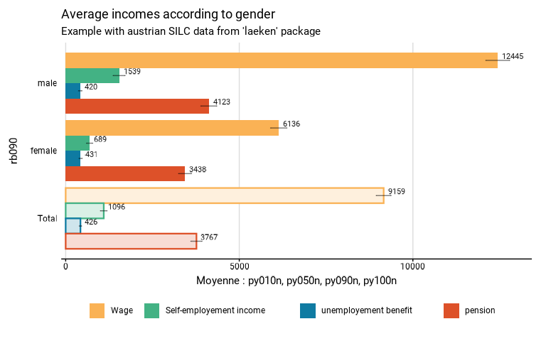
eusilc_many_mean_group <- many_mean_group(
eusilc,
group = rb090,
list_vars = c(py010n,py050n,py090n,py100n),
list_vars_lab = c("Wage","Self-employement income","unemployement benefit","pension"),
strata = db040,
ids = db030,
weight = rb050,
title = "Average incomes according to gender",
subtitle = "Example with austrian SILC data from 'laeken' package"
)
#> Variables used: py010n, py050n, py090n, py100n
#> Input: data.frame
#> Sampling design -> ids: db030, strata: db040, weights: rb050
#> Numbers of observation(s) removed by each filter (one after the other):
#> 0 observation(s) removed due to missing group
#> Warning: With na.vars = 'rm', observations removed differ between variables
#>
#> Attaching package: 'srvyr'
#> The following object is masked from 'package:stats':
#>
#> filter
# Results in graph form
eusilc_many_mean_group$graph
#> Warning: Removed 8 rows containing missing values or values outside the scale range
#> (`geom_bar()`).
#> Warning: Removed 8 rows containing missing values or values outside the scale range
#> (`geom_text()`).
#> Warning: Removed 4 rows containing missing values or values outside the scale range
#> (`geom_text()`).
 # Results in table format
eusilc_many_mean_group$tab
#> # A tibble: 12 × 9
#> rb090 list_col mean mean_low mean_upp n_sample n_weighted n_weighted_low
#> <fct> <fct> <dbl> <dbl> <dbl> <int> <dbl> <dbl>
#> 1 male Wage 12445. 12102. 12787. 5844 3237897. 3178503.
#> 2 female Wage 6136. 5902. 6370. 6263 3519368. 3470221.
#> 3 Total Wage 9159. 8946. 9372. 12107 6757264. 6683738.
#> 4 male Self-empl… 1539. 1369. 1710. 5844 3237897. 3178503.
#> 5 female Self-empl… 689. 600. 778. 6263 3519368. 3470221.
#> 6 Total Self-empl… 1096. 1002. 1191. 12107 6757264. 6683738.
#> 7 male unemploye… 420. 371. 469. 5844 3237897. 3178503.
#> 8 female unemploye… 431. 387. 475. 6263 3519368. 3470221.
#> 9 Total unemploye… 426. 393. 458. 12107 6757264. 6683738.
#> 10 male pension 4123. 3894. 4353. 5844 3237897. 3178503.
#> 11 female pension 3438. 3254. 3623. 6263 3519368. 3470221.
#> 12 Total pension 3767. 3606. 3927. 12107 6757264. 6683738.
#> # ℹ 1 more variable: n_weighted_upp <dbl>
# Results in table format
eusilc_many_mean_group$tab
#> # A tibble: 12 × 9
#> rb090 list_col mean mean_low mean_upp n_sample n_weighted n_weighted_low
#> <fct> <fct> <dbl> <dbl> <dbl> <int> <dbl> <dbl>
#> 1 male Wage 12445. 12102. 12787. 5844 3237897. 3178503.
#> 2 female Wage 6136. 5902. 6370. 6263 3519368. 3470221.
#> 3 Total Wage 9159. 8946. 9372. 12107 6757264. 6683738.
#> 4 male Self-empl… 1539. 1369. 1710. 5844 3237897. 3178503.
#> 5 female Self-empl… 689. 600. 778. 6263 3519368. 3470221.
#> 6 Total Self-empl… 1096. 1002. 1191. 12107 6757264. 6683738.
#> 7 male unemploye… 420. 371. 469. 5844 3237897. 3178503.
#> 8 female unemploye… 431. 387. 475. 6263 3519368. 3470221.
#> 9 Total unemploye… 426. 393. 458. 12107 6757264. 6683738.
#> 10 male pension 4123. 3894. 4353. 5844 3237897. 3178503.
#> 11 female pension 3438. 3254. 3623. 6263 3519368. 3470221.
#> 12 Total pension 3767. 3606. 3927. 12107 6757264. 6683738.
#> # ℹ 1 more variable: n_weighted_upp <dbl>