Function that represents the values of a group variable as areas proportional to those values.
Usage
make_surface(
  tab,
  var,
  value,
  error_low = NULL,
  error_upp = NULL,
  facet = NULL,
  pvalue = NULL,
  reorder = FALSE,
  compare = FALSE,
  space = NULL,
  position = "mid",
  show_ci = TRUE,
  name_total = "Total",
  digits = 0,
  unit = NULL,
  col = NULL,
  pal = "OBSS_Autumn",
  direction = 1,
  desaturate = 0,
  lighten = 0,
  darken = 0,
  size_text = 3.88,
  bg = "#f8f5f5",
  linewidth_ci = 0.5,
  ratio = 3/2,
  font = "Roboto",
  wrap_width_lab = 20,
  title = NULL,
  subtitle = NULL,
  hjust.title = 0,
  caption = NULL,
  coef_font = 1
)
Arguments
- tab
dataframe with the variables to be ploted.
- var
The variable in
tabwith the labels of the indicator to be ploted.- value
The variable in
tabwith the values of the indicator to be ploted.- error_low
The variable in
tabthat is the lower bound of the confidence interval. If eithererror_loworerror_uppisNULLerror rectangles are not shown on the graphic.- error_upp
The variable in
tabthat is the upper bound of the confidence interval. If eithererror_loworerror_uppisNULLerror rectangles are not shown on the graphic.- facet
A variable in
tabdefining the faceting group, if applicable. Default isNULL.- pvalue
The p-value to show in the caption. It can be a numeric value or the pvalue object from a statistical test.
- reorder
TRUEif you want to reorder the values.NAlabel invaris not included in the reorder.- compare
TRUEto display a rectangle representing the smallest value. When facets are enabled, this is the smallest value per facet category.- space
The space between the rectangles. The unit is that of the indicator.
- position
The position of the rectangles:
"mid"for center alignment,"bottom"for bottom alignment.- show_ci
TRUEif you want to show the CI on the graphic. The bounds of the confidence intervals are displayed as dotted rectangles around the result.FALSEif you do not want to show them. Default isTRUE.- name_total
Name of the
varlabel that may contain the total. When indicated, it is not displayed on the graph.- digits
Number of decimal places displayed on the values labels on the graphic. Default is
0.- unit
The unit showd on the plot. Default is none (
"").- col
Color of the rectangles if the user wants a monocolor graph.
colmust be a R color or an hexadecimal color code. Aspalhas a priority overcol, if the user wants to usecol, he must not use simultaneously thepalargument (evenpal = NULL).- pal
Colors of the rectangles if the user wants the rectangles to have different colors.
palmust be vector of R colors or hexadecimal colors or a palette from packages MetBrewer or PrettyCols or a palette from fonctionr.palhas a priority overcol.- direction
Direction of the palette color. Default is
1. The opposite direction is-1.- desaturate
Numeric specifying the amount of desaturation where
1corresponds to complete desaturation (no colors, grey layers only),0to no desaturation, and values in between to partial desaturation. Default is0. It affects only the palette (pal) and not the monocolor (col). Seecolorspace::desaturate()for details. If desaturate and lighten/darken arguments are used, lighten/darken is applied in a second time (i.e. on the color transformed by desaturate).- lighten
Numeric specifying the amount of lightening. Negative numbers cause darkening. Value shoud be ranged between
-1(black) and1(white). Default is0. It affects only the palette (pal) and not the monocolor (col). Seecolorspace::lighten()for details. If both argument ligthen and darken are used (not advised), darken is applied in a second time (i.e. on the color transformed by lighten).- darken
Numeric specifying the amount of lightening. Negative numbers cause lightening. Value shoud be ranged between
-1(white) and1(black). Default is0. It affects only the palette (pal) and not the monocolor (col). Seecolorspace::darken()for details. If both argument ligthen and darken are used (not advised), darken is applied in a second time (i.e. on the color transformed by lighten).- size_text
Text size displayed in rectangles . Default is
3.88(as in ggplot2).- bg
Color of the background.
bgmust be a R color or an hexadecimal color code.- linewidth_ci
Line width of the dotted confidence intervals lines. It affects also the lenghts of the dots and spaces bteween dots. Default is
0.5to have confidence lines two times thiner than the lines of the indicators.- ratio
Ratio between the length and the width of the rectangles.
1produces squares ; greater than1produces vertical rectangles and smaller than1produces horizontal rectangles. Default is3/2.- font
Font used in the graphic. See
load_and_active_fonts()for available fonts. Default is"Roboto".- wrap_width_lab
Number of characters before going to the line for the labels of the categories of
var. Default is20.- title
Title of the graphic.
- subtitle
Subtitle of the graphic.
- hjust.title
Horizontal alignment of title & subtitle. It should take a numeric value. Default (
0) leads to left alignment,1leads to right alignment and0.5leads to centered alignement.- caption
Caption of the graphic.
- coef_font
A multiplier factor for font size of all fonts on the graphic. Default is
1. Usefull when exporting the graphic for a publication (e.g. in a Quarto document).
Examples
# Loading of data
data(eusilc, package = "laeken")
# Recoding eusilc$pl030 into eusilc$pl030_rec
eusilc$pl030_rec <- NA
eusilc$pl030_rec[eusilc$pl030 == "1"] <- "Working full time"
eusilc$pl030_rec[eusilc$pl030 == "2"] <- "Working part time"
eusilc$pl030_rec[eusilc$pl030 == "3"] <- "Unemployed"
eusilc$pl030_rec[eusilc$pl030 == "4"] <- "Student"
eusilc$pl030_rec[eusilc$pl030 == "5"] <- "Retired"
eusilc$pl030_rec[eusilc$pl030 == "6"] <- "Permanently disabled"
eusilc$pl030_rec[eusilc$pl030 == "7"] <- "Fulfilling domestic tasks"
# Calculation of income means by age category with fonctionr, taking sample design into account
eusilc_mean <- mean_group(
eusilc,
group = pl030_rec,
quanti_exp = py010n + py050n + py090n + py100n + py110n + py120n + py130n + py140n,
filter_exp = !pl030_rec %in% c("Student", "Fulfilling domestic tasks") & db040 == "Tyrol",
weights = rb050
)
#> Input: data.frame
#> Sampling design -> ids: `1`, weights: rb050
#> Variable(s) detected in quanti_exp: py010n, py050n, py090n, py100n, py110n, py120n, py130n, py140n
#> Numbers of observation(s) removed by each filter (one after the other):
#> 13680 observation(s) removed by filter_exp
#> 296 observation(s) removed due to missing group
#> 0 observation(s) removed due to missing value(s) for the variable(s) in quanti_exp
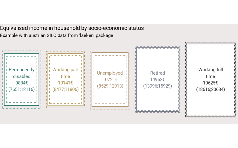
# Displaying results with make_surface()
eusilc_mean$tab |>
make_surface(
var = pl030_rec,
value = mean,
error_low = mean_low,
error_upp = mean_upp,
reorder = TRUE,
wrap_width_lab = 15,
unit = "€",
title = "Equivalised income in household by socio-economic status",
subtitle = "Example with austrian SILC data from 'laeken' package"
)